
Finer
Halves the channel-start area: more headwater branches, smaller sub-basins.
Features
Point Cloud Viewer Point Cloud Preprocessing Point Cloud Classification Point Cloud Rasterization Point Cloud Vectorization Photogrammetry Processing APIIndustry
Land Surveying Utility Vegetation Management Forestry Hydrology & WaterMore
Pricing Contact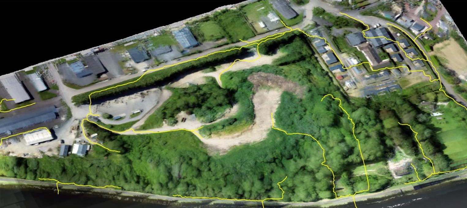
LiDAR for hydrology
Flow accumulation, drainage axes, closed depressions, sub-basins, water bodies and shorelines — derived from your own survey and delivered as vectors, rasters and CAD layers.
No software to install • 50 hectares included
The challenge
The terrain model is the easy half. Turning it into a drainage network usually means a desktop GIS, a chain of tools run by hand, and a threshold nobody can defend.
The layers
Flow accumulation
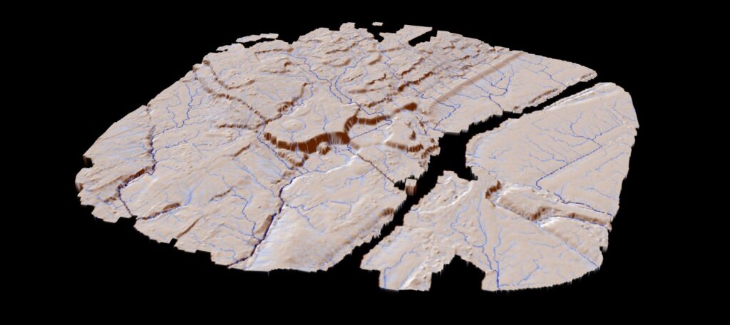
A catchment-area raster over hillshaded terrain.
Every cell carries the area that drains through it, computed on a hydrologically conditioned surface built from your ground points. The display raster shades the whole field on a logarithmic ramp over a hillshade of that surface, so the network reads against the relief that produces it instead of floating on a flat background.
Drainage axes
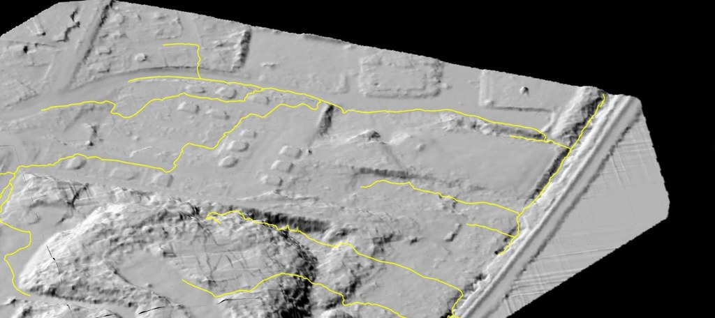
One 3D line per stream link, carrying what it drains.
The network above the channel-start threshold is split into links, Strahler-ordered, smoothed and traced along the conditioned surface. Every vertex carries an elevation, so the axes sit on the terrain in the 3D viewer and come into CAD as 3D polylines rather than flat lines you have to drape yourself.
Depressions
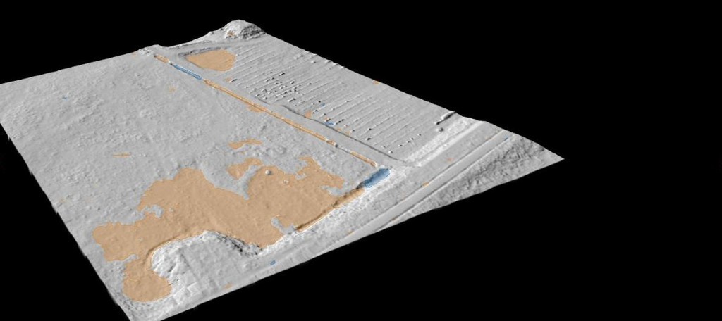
Depth, volume and spill level for every basin that holds water.
Depressions are computed on the raw ground surface, before conditioning, so what you receive is the hollow as it was surveyed rather than the remainder left after an algorithm smoothed the terrain. Each polygon records how deep it is, how much it holds, and how the conditioning treated it.
Sub-basins
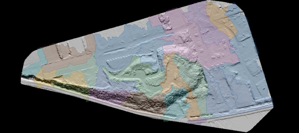
The survey divided into the area feeding each stream outlet.
The site is split into the drainage area that feeds each outlet of the network and clipped to the surveyed footprint. Basins below a usable size are dissolved into the one downstream, so you get catchments you can work with rather than one polygon per pixel.
Detail
The channel-start threshold is derived from the surveyed area, the median slope and the surface noise measured on your own cloud. A single setting shifts the whole ladder when you want a denser or a sparser network.
Halves the channel-start area: more headwater branches, smaller sub-basins.
The default. The threshold follows the site, and steeper ground lowers it on its own.
Doubles it: the main network only, and larger catchments behind it.
Water surfaces
Water bodies & shorelines
Enclosed water closes into a polygon; water that leaves the survey opens into a shoreline.
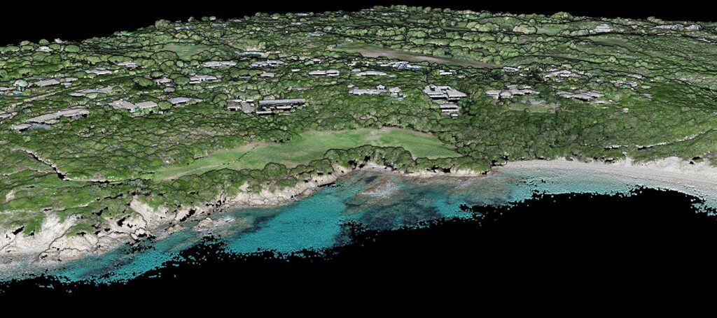
Water is found on the orthophoto and then grown against the point cloud itself, so the boundary follows the water surface rather than a colour edge in a photograph. Water fully enclosed inside the surveyed area closes into a polygon; water that runs out of coverage opens into shoreline lines instead — a river gets two banks, a coast gets one.
CAD
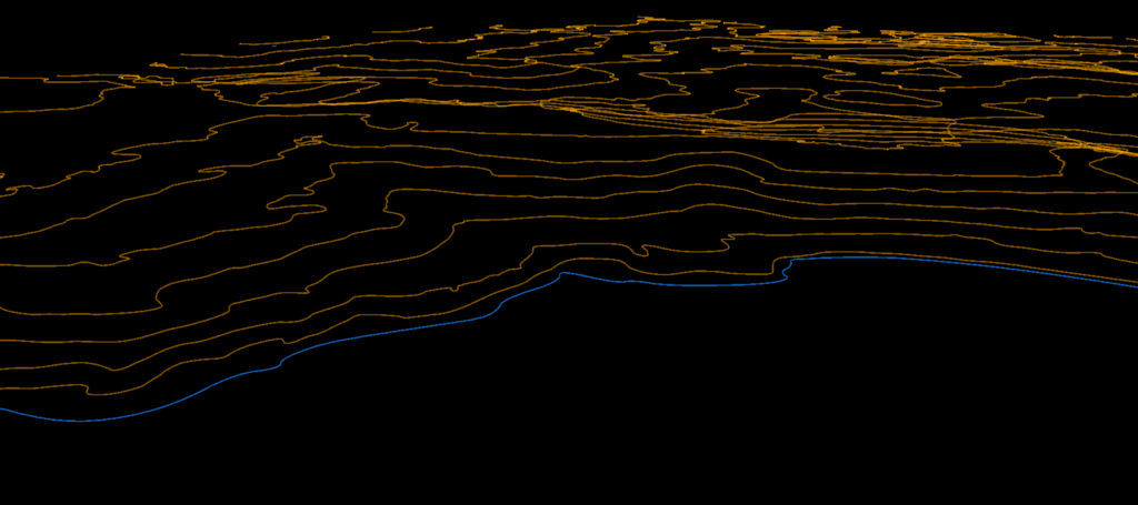
Hydrography arrives as its own layers in the topographic map.
Drainage axes, depressions and sub-basins each land on their own layer in the topographic-map DXF, beside the shoreline, the water body and the contours. The sheet legend is generated with them, and the printable PDF comes out of the same drawing.
Reference
| Layer | Geometry | Attributes | Formats |
|---|---|---|---|
| Flow accumulation | Raster | Catchment area per cell, plus the conditioned surface | GeoTIFF |
| Drainage axes | 3D lines | Order, upstream area, length, slope, edge flag | GeoJSON, SHP, DXF |
| Depressions | 3D rings | Max and mean depth, area, volume, spill level, treatment, edge flag | GeoJSON, SHP, DXF |
| Sub-basins | 3D rings | Area, outlet order, outlet X/Y/Z, edge flag | GeoJSON, SHP, DXF |
| Water body | Polygons | Type, islands as holes | GeoJSON, SHP, DXF |
| Shoreline | Lines | Type | GeoJSON, SHP, DXF |
GeoJSON is written in WGS 84; shapefiles and DXF stay in your project CRS. On a survey in feet, areas and lengths are converted with the file.
How it works
Drag and drop LAS or LAZ files, with your orthophoto if you have one. No conversion, no preprocessing.
Tick the layers you need — flow accumulation, axes, depressions, sub-basins, water body, shoreline — and pick a level of detail.
Inspect everything in the 3D viewer, then download the vectors, the rasters, the CAD drawing and the report.
Outputs
Every vector layer in WGS 84, ready for web maps and for GIS.
SHP with its DBF, SHX and PRJ, in your project CRS, attributes included.
One drawing per layer, plus the merged topographic map with all of them on it.
Flow accumulation and the conditioned terrain surface, georeferenced.
Every layer standing on the terrain in the browser, attributes on hover.
A hydrology section in the PDF: counts, lengths, volumes and the parameters used.
Use cases
Concentration paths and contributing areas measured on the surveyed ground, not on an open-data terrain model.
Where water reaches a road, a platform or a trench, and which hollows will hold it afterwards.
Depth, area and volume for every closed hollow, with the level at which it spills.
Shorelines and water bodies as survey vectors, with the water surface classified in the cloud.
Questions
No. The hydrology stage builds its own ground surface from the classified point cloud, at a resolution chosen from the size of the surveyed area. You do not have to run the DTM first, and turning the DTM off does not turn hydrology off.
A raw ground surface has hollows that water cannot leave, so a flow algorithm stalls in them. The hydrology stage first breaches a hollow where a genuine outlet lies close enough, then fills whatever is left, and runs the flow analysis on that surface. It is delivered as its own raster beside the flow accumulation. Your DTM deliverable is untouched, and no watercourse is ever burned into the terrain.
From your site rather than from a default. It scales with the surveyed area, drops on steep ground and rises on flat ground, and is bounded at both ends so a very small or very large survey still gets a sensible network. The Finer and Coarser settings halve and double it. The value actually used is written into the report and into the layer metadata.
Because a survey has a boundary and water does not. A stream that enters from outside the flown area carries a catchment we cannot see, and a basin touching the boundary is only the part inside it. Those features are flagged so you can tell a measured catchment from a truncated one instead of quietly under-reporting it.
It works best with one. Water is detected on imagery and then grown against the point cloud, so an orthophoto of your own survey gives the sharpest result. When you have none, you can allow the use of open satellite imagery for the detection step, and the extraction still runs against your cloud. If you upload the photos of your flight, the orthophoto built from them is the one used, see photogrammetry.
Yes. The vectors are editable in the viewer like every other vector deliverable, and regenerating the report and the topographic map after an edit rebuilds the drawing with your changes on it.
Documentation
How to process water and drainage layers with Lidarvisor.
Upload a survey, tick the layers you need, and get the drainage network, the hollows and the catchments back with the rest of your deliverables.
Get started freeNo software to install. No thresholds to guess. View pricing or contact our team