Airborne survey systems, outputs, and processing workflows
What Is Airborne LiDAR?
Airborne LiDAR (Light Detection and Ranging) is a remote sensing technology that captures precise three-dimensional measurements of the Earth’s surface from aircraft. Unlike ground-based survey methods that measure terrain point by point, airborne LiDAR systems emit millions of laser pulses per second from fixed-wing aircraft, helicopters, or drones, creating dense point clouds that reveal surface details invisible to traditional imaging.
The technology works by measuring the time it takes for laser pulses to travel from the sensor to the ground and back. With pulses fired at rates exceeding 2 MHz (2 million per second), modern systems generate point densities of 8-100+ points per square meter, depending on altitude and flight parameters.
What makes airborne LiDAR particularly valuable is its ability to penetrate vegetation. Unlike photogrammetry, which captures only visible surfaces, LiDAR pulses pass through gaps in tree canopy to reach the ground. A single pulse can register multiple returns: first from the canopy top, intermediate returns from mid-story vegetation, and a final return from the bare earth below.
The Evolution of Airborne LiDAR
Airborne LiDAR emerged from military laser rangefinder technology in the 1970s. NASA’s Airborne Oceanographic Lidar, deployed in 1978, was among the first operational systems.
First-generation systems achieved pulse rates of 2,000-10,000 Hz with positioning accuracy measured in meters. By the 2000s, pulse rates reached 100 kHz and positioning improved to decimeter levels. Today’s sensors fire at 2+ MHz with centimeter-level accuracy.
The miniaturization of LiDAR sensors has been equally dramatic. Systems that once required twin-engine aircraft now fit on consumer drones, expanding airborne LiDAR from government mapping programs to everyday surveying applications.
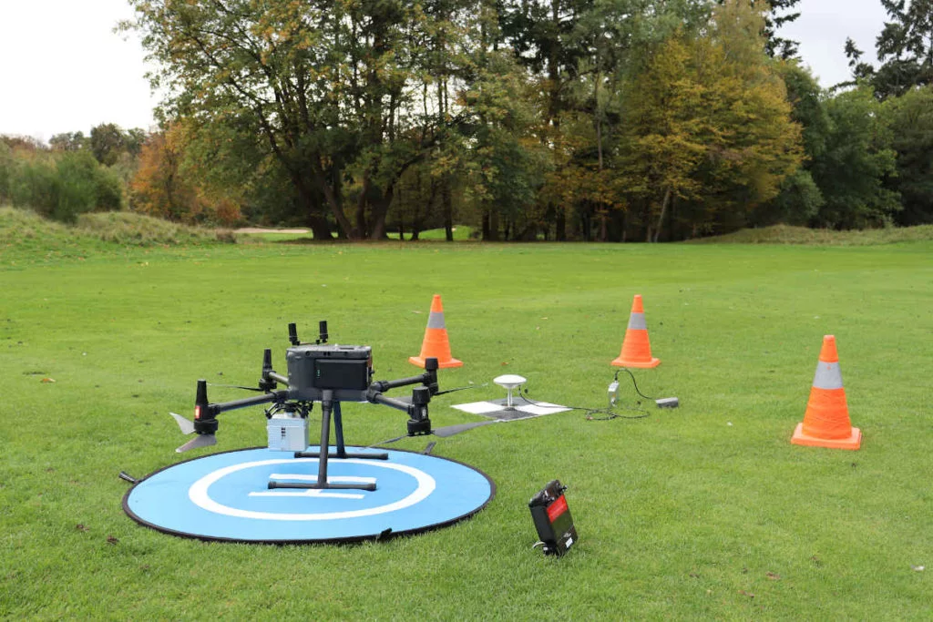
Modern drone-mounted LiDAR systems have democratized airborne surveying
Core Components of Airborne LiDAR Systems
Multiple Returns and Full Waveform LiDAR
When a laser pulse encounters vegetation, it doesn’t simply bounce back from a single surface. The pulse interacts with multiple surfaces along its path.
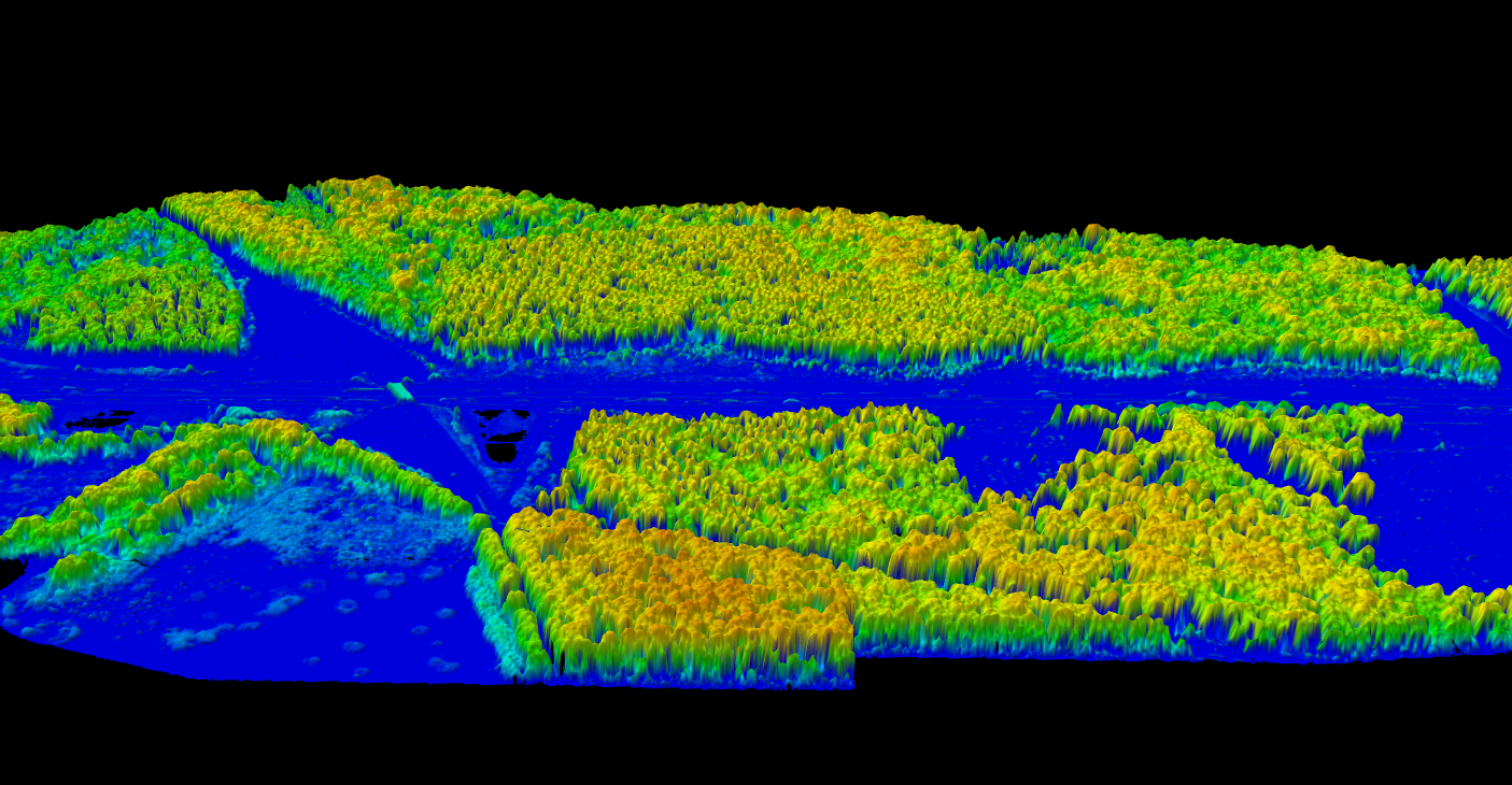
3D Canopy Height Model showing vegetation structure from ground to canopy top — generated from LiDAR multiple returns
Discrete Return Systems
Most commercial systems record “discrete returns,” detecting distinct peaks in the reflected signal. A pulse passing through a forest might register:
✦ First return: Top of canopy
✦ Second return: Mid-canopy branch layer
✦ Third return: Understory vegetation
✦ Last return: Ground surface
Full Waveform Systems
Full waveform LiDAR digitizes the entire reflected signal rather than just detecting peaks. This produces a continuous record of energy return over time, revealing:
✦ Subtle canopy structure variations
✦ Vegetation density mapping
✦ Surface characteristics
✦ Biomass estimation
Types of Airborne LiDAR Platforms
✈️
Fixed-Wing Aircraft
Workhorse of large-area mapping
Altitude: 500-4,000 m AGL
Point density: 1-25 pts/m²
Coverage: 100-500 km²/day
Accuracy: 5-15 cm RMSE
🚁
Helicopter Systems
Flexibility for corridors & urban
Altitude: 150-1,500 m AGL
Point density: 10-50 pts/m²
Coverage: 20-100 km²/day
Accuracy: 3-10 cm RMSE
🛸
Drone (UAV) LiDAR
Ultra-high density for small sites
Altitude: 30-150 m AGL
Point density: 50-400+ pts/m²
Coverage: 2-30 ha/flight
Accuracy: 2-5 cm RMSE
Platform Selection Guide
| Parameter | Fixed-Wing | Helicopter | Drone |
|---|---|---|---|
| Project size sweet spot | >500 ha | 50-1,000 ha | 5-100 ha |
| Point density | 1-25 pts/m² | 10-50 pts/m² | 50-400 pts/m² |
| Mobilization cost | High ($10-30k) | High ($5-20k) | Low ($0-2k) |
| Per-hectare (large) | Lowest | Medium | Highest |
| Terrain flexibility | Limited | High | Highest |
Key Applications of Airborne LiDAR
PROCESSING WORKFLOW
Airborne LiDAR Data Processing
Raw LiDAR data requires several processing stages before generating usable deliverables:
Teams comparing drone LiDAR processing and mobile LiDAR processing can use the same classification and export workflow once the airborne point cloud is uploaded.
1. Trajectory Processing — GNSS and IMU data combined for precise aircraft position
2. Point Cloud Generation — Georeferenced XYZ points with intensity and return data
3. Quality Control — Density, overlap, and accuracy verification
4. Classification — Assigning points to ground, vegetation, buildings, etc.
5. Product Generation — DTM, DSM, CHM, contours, and derivatives
6. Delivery — LAS/LAZ, GeoTIFF, shapefiles in standard formats
Point Cloud Classification
Classification assigns each point to a feature category. The ASPRS LAS specification defines standard classes:
| Class | Description |
|---|---|
| 2 | Ground |
| 3-5 | Low, Medium, High Vegetation |
| 6 | Building |
| 9 | Water |
| 14 | Wire (Conductor) |
| 15 | Transmission Tower |
Traditional classification required manual editing in desktop software, often taking days to weeks. Lidarvisor automates classification using machine learning, identifying ground, vegetation, buildings, water, wires, poles, towers, and other features without manual intervention.
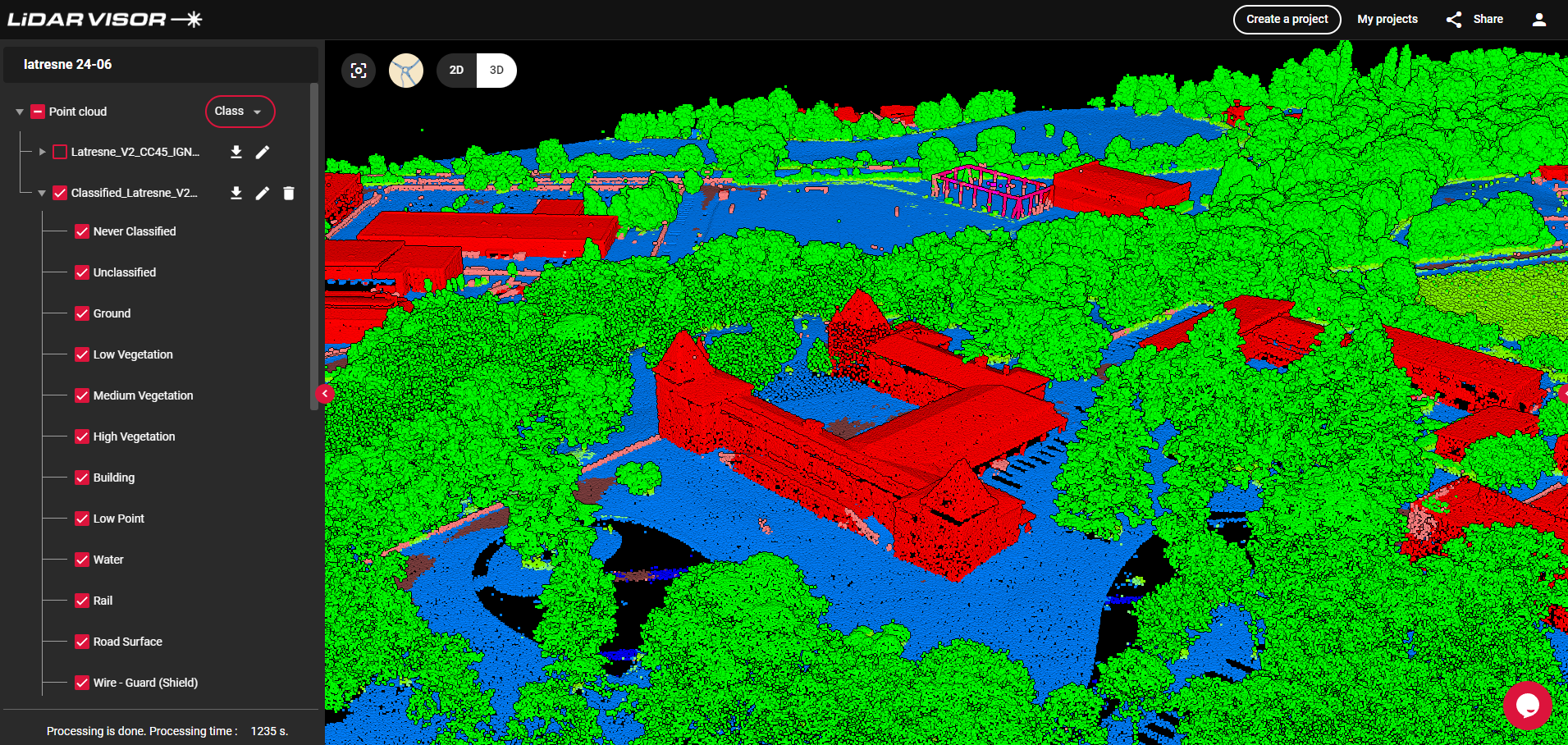
Lidarvisor’s cloud-based classification interface — automatically classify and visualize point clouds
Airborne vs. Terrestrial vs. Mobile LiDAR
Airborne LiDAR
Coverage: 10-500 km²/day
Density: 1-100 pts/m²
Accuracy: 3-15 cm RMSE
Best for: Large areas, inaccessible terrain, vegetation penetration
Terrestrial LiDAR
Coverage: 0.1-1 ha/day
Density: 1,000-100,000 pts/m²
Accuracy: 1-5 mm
Best for: Building interiors, complex structures, heritage, forensics
Mobile LiDAR
Coverage: 20-100 km/day
Density: 100-2,000 pts/m²
Accuracy: 1-3 cm
Best for: Road corridors, railways, urban streets, indoor spaces
Classified Point Cloud Example
This classified point cloud shows a rural area with forest, captured by airborne LiDAR. Different colors represent different classification categories:
- Brown — Ground points (bare earth)
- Green — Vegetation (low, medium, high)
- Tan — Buildings and structures
Multiple returns through the forest canopy allow the algorithm to distinguish ground from vegetation, enabling accurate DTM extraction even in dense forest areas.
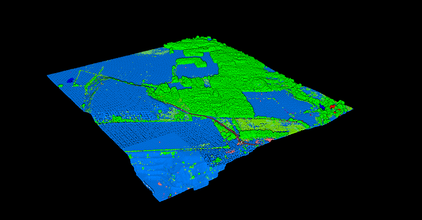
Classified airborne LiDAR point cloud — rural area with forest
Cost Considerations
Fixed-Wing Surveys:
- Large area (>1,000 km²): $100-300 per km²
- Medium area (100-1,000 km²): $200-500 per km²
- Small area (<100 km²): $500-1,500 per km² due to fixed mobilization costs
Helicopter Surveys:
- Corridor mapping: $500-2,000 per linear km at 25+ pts/m²
- Area surveys: $400-800 per km² for high-density acquisition
Drone LiDAR:
- Per-hectare rates: $50-300 depending on terrain and density
- Day rate: $2,000-5,000 per day covering 10-50 hectares
Processing Costs: Data processing historically represented 40-60% of total project cost when performed manually. Automated classification through Lidarvisor can reduce processing time dramatically, shifting the cost balance toward acquisition.
Frequently Asked Questions
Airborne LiDAR actively emits laser pulses to measure distances directly, while photogrammetry derives 3D data from overlapping photographs. Key differences: LiDAR penetrates vegetation canopy (photogrammetry only sees visible surfaces), LiDAR works in darkness (photogrammetry requires good lighting), and LiDAR measures range directly (photogrammetry interpolates from image correlation). Many projects now combine both technologies.
Modern airborne systems achieve 5-15 cm vertical accuracy (RMSE) and 15-30 cm horizontal accuracy on hard, flat surfaces. Accuracy degrades in vegetation due to ground detection uncertainty. Drone LiDAR at low altitude can achieve 2-5 cm vertical accuracy.
LiDAR pulses pass through gaps in canopy to reach the ground. In deciduous forest during leaf-off conditions, ground penetration exceeds 90%. In dense coniferous or tropical forest, 20-40% of pulses may reach the ground. Multiple-return capability ensures even partial penetration captures ground points. Higher point density increases probability of ground hits.
Traditional manual processing can take days to weeks depending on project size and classification complexity. A 100 km² project might require 40-80 hours of technician time for full classification. Automated processing through Lidarvisor reduces turnaround dramatically for classification, DTM/DSM generation, and feature extraction.
The industry-standard format is LAS (ASPRS LAS Specification) and its compressed variant LAZ. These formats store XYZ coordinates, intensity, return information, classification, and metadata. LAS 1.4 supports extended point formats with additional attributes. Raster products (DTM, DSM) typically use GeoTIFF format. Cloud-optimized formats (COPC, COG) enable streaming access to large datasets.
LiDAR requires clear air between sensor and ground. Clouds, fog, and heavy rain absorb or scatter laser pulses, preventing data collection. Light rain and haze may reduce range but allow acquisition at lower altitudes. Snow cover is acceptable if terrain (not snow surface) is the target. Leaf-off conditions in deciduous forests improve ground penetration significantly.